This article explains a breif introduction of CNN and about how to build a model to classify images of clothing (like T-shirt, Trouser) using it in TensorFlow. If you are beginner, I would recommend to read following posts first:

- Setup Deep Learning environment: Tensorflow, Jupyter Notebook and VSCode

- Tensorflow 2: Build Your First Machine Learning Model with tf.keras

CNN

As the name "convolutional neural network" implies, it uses mathematical operation called Convolution for image input. In image processing, a kernel is a small matrix and it is applied to an image with convolution operator.

Kernal slides over the input matrix, applies a pair-wise multipication of two matrixes and the sum the multipication output and put into the resultant matrix.

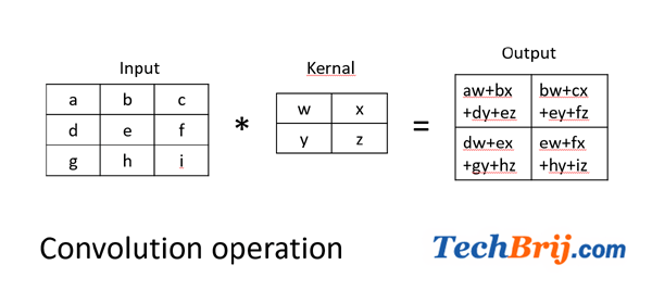
Let's understand it with an example:

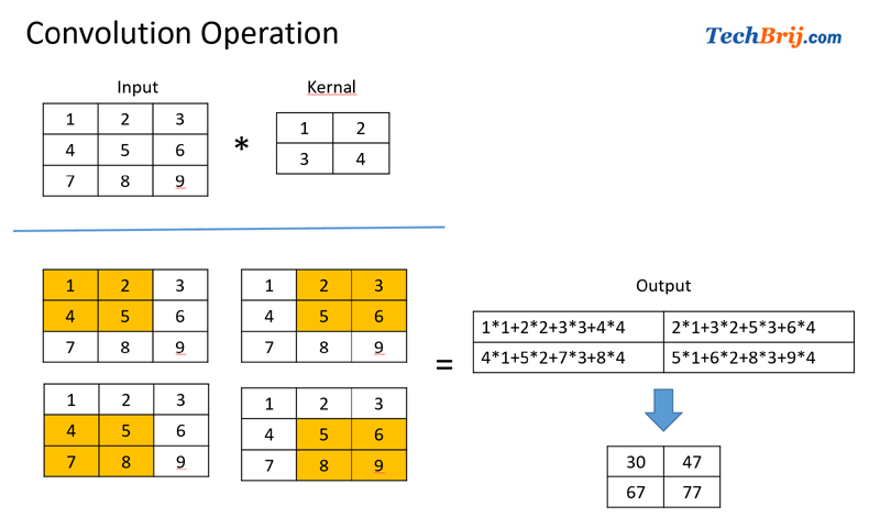
Strides: Stride is the number of pixels shifts over the input matrix. When the stride is 1 then we move the filters to 1 pixel at a time. When the stride is 2 then we move the filters to 2 pixels at a time and so on.

Padding: Sometimes filter does not fit perfectly fit the input image. We have two options:

- Pad the picture with zeros (zero-padding) so that it fits

- Drop the part of the image where the filter did not fit. This is called valid padding which keeps only valid part of the image.

Now the question is how Convolution is used in image processing? Here input is image pixel and kernal is used to applying a filter to an image extracts some features from it. Convolution of an image with different filters can perform operations such as edge detection, blur and sharpen by applying filters.

CNN is widely used for images recognition, images classifications, Objects detections, recognition faces etc.

CNN Layers

CNN Architecture has different layers.

Input Layer:

It holds the raw input of image with generally a particular width x height x depth.

Convolutional layer:

It is used to extract features from an input image. The layer's parameters consist of a set of learnable filters (or kernels). Each filter is convolved across the width and height of the input volume, computing the dot product between the entries of the filter and the input and producing a 2-dimensional activation map of that filter. As a result, the network learns filters that activate when it detects some specific type of feature at some spatial position in the input.

Generally, ReLU stands for Rectified Linear Unit for a non-linear operation is used as activation function. The output is ƒ(x) = max(0,x).

Pooling Layer:

It is used to reduce the number of parameters when the images are too large. Common types of pooling layers are max pooling, average pooling and sum pooling.

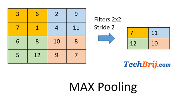
Max pooling takes the largest element from the rectified feature map.

If we use a max pool with 2 x 2 filters and stride 2, here is an example with 4x4 input:

Fully-Connected Layer:

It is regular neural network layer which takes input from the previous layer and computes the class scores and outputs the 1-D array of size equal to the number of classes.

Dataset

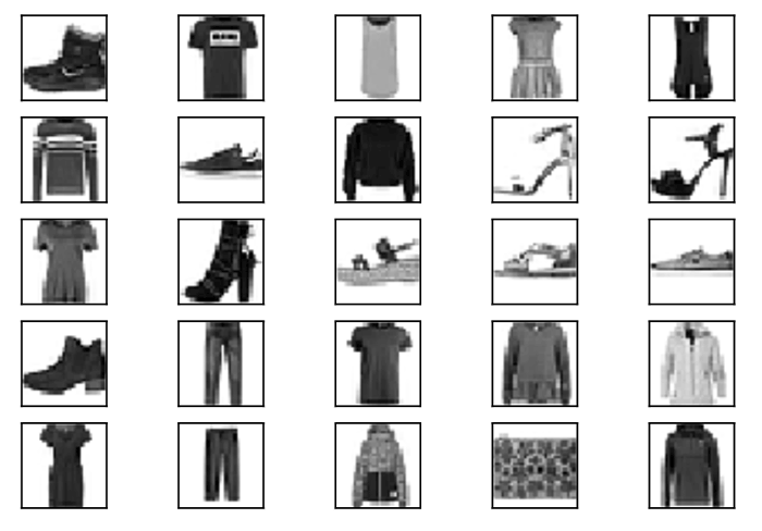
We will train a convolutional neural network to classify clothes types from the Fashion MNIST dataset. Let's import the modules first:

import tensorflow as tf
import matplotlib.pyplot as plt
import numpy as np

use following code to load fashion MNIST data:

fashion_mnist = tf.keras.datasets.fashion_mnist
(x_train, y_train), (x_test, y_test) = fashion_mnist.load_data()

First time, it will download the datasets.

Let's define the class name and visualize few data:

class_names = ['T-shirt/top', 'Trouser', 'Pullover', 'Dress', 'Coat',
               'Sandal',      'Shirt',   'Sneaker',  'Bag',   'Ankle boot']

# plot first few images
for i in range(25):    
    # define subplot
    plt.subplot(5, 5, i+1)
    plt.grid(False)
    plt.xticks([])
    plt.yticks([])
    # plot raw pixel data
    plt.imshow(x_train[i], cmap=plt.cm.binary)
    
# show the figure
plt.show()

Without CNN

In my aricle, we did image classification on handwritten digits. Let's use the same way of classification here and see the results.

# resize image
x_train, x_test = x_train / 255.0, x_test / 255.0

# model
model = tf.keras.models.Sequential([
  tf.keras.layers.Flatten(input_shape=(28, 28)),
  tf.keras.layers.Dense(128, activation='relu'),
  tf.keras.layers.Dropout(0.2),
  tf.keras.layers.Dense(10, activation='softmax')
])

# compile the model
model.compile(optimizer='adam',
              loss='sparse_categorical_crossentropy',
              metrics=['accuracy'])
			  
# train the model
model.fit(x_train, y_train, epochs=5)

# evaluate the model
model.evaluate(x_test,  y_test, verbose=2)

Output:

[0.352192257642746, 0.8756]

means testing accuracy is ~87%.

Let's see to get prediction on first test image

img =  np.array([x_test[0]])
 predictions = model.predict(img) 
 predicted_class = np.argmax(predictions[0])
 original_class = y_test[0]
 print('Original class: {} \nPredicted class: {}'.format(original_class, predicted_class))

Output:

Original class: 9 
Predicted class: 9

which looks good.

With CNN

Let's update the program to use CNN approach. First preprocess the data to resize image and scale the pixel values from the default range of 0-255 to 0-1

X_train_final = x_train.reshape((-1, 28, 28, 1)) / 255.
X_test_final = x_test.reshape((-1, 28, 28, 1)) / 255.

Let's define and compile the model:

# define the model
model_with_conv = tf.keras.Sequential([
    tf.keras.layers.Conv2D(32, (3,3), padding='same', activation=tf.nn.relu, input_shape=(28, 28, 1)),
    tf.keras.layers.MaxPooling2D((2, 2), strides=2),
    tf.keras.layers.Conv2D(64, (3,3), padding='same', activation=tf.nn.relu),
    tf.keras.layers.MaxPooling2D((2, 2), strides=2),
    tf.keras.layers.Flatten(),    
    tf.keras.layers.Dense(128, activation=tf.nn.relu),
    #  10-node softmax layer, with each node representing a class of clothing.
    tf.keras.layers.Dense(10,  activation=tf.nn.softmax)
])

# compile the model
model_with_conv.compile(optimizer='adam',
              loss='sparse_categorical_crossentropy',
              metrics=['accuracy'])

Here neural network start with two pairs of Conv/MaxPool.

- The first layer is a Conv2D filters (3,3) being applied to the input image, retaining the original image size by using padding, and creating 32 output (convoluted) images (so this layer creates 32 convoluted images of the same size as input).

- After that, the 32 outputs are reduced in size using a MaxPooling2D (2,2) with a stride of 2.

- The next Conv2D also has a (3,3) kernel, takes the 32 images as input and creates 64 outputs which are again reduced in size by a MaxPooling2D layer.

- In output dense layers, a 128-neuron, followed by 10-node softmax layer. Each node represents a class of clothing.

Let's train and evaluate the model:

model_with_conv.fit(X_train_final, y_train, epochs=5)
model_with_conv.evaluate(X_test_final,  y_test, verbose=2)

Output:

[0.24095578503012657, 0.9162]

Test accuracy is ~92%. We can clearly see improvement in accuracy. Without CNN it was approx 87%.

Let's get prediction on some test images and visualize the result:

def plot_image(i, predictions_array, true_labels, images):
  predictions_array, true_label, img = predictions_array[i], true_labels[i], images[i]
  plt.grid(False)
  plt.xticks([])
  plt.yticks([])
  
  plt.imshow(img[...,0], cmap=plt.cm.binary)

  predicted_label = np.argmax(predictions_array)
  if predicted_label == true_label:
    color = 'blue'
  else:
    color = 'red'
  
  plt.xlabel("{} {:2.0f}% ({})".format(class_names[predicted_label],
                                100*np.max(predictions_array),
                                class_names[true_label]),
                                color=color)
								
								
								
# Plot the first X test images, their predicted label, and the true label
# Color correct predictions in blue, incorrect predictions in red
num_rows = 5
num_cols = 5
num_images = num_rows*num_cols
plt.figure(figsize=(2*num_cols, 2*num_rows))
test_images = X_test_final[:num_images]
predictions = model_with_conv.predict(test_images)
for i in range(num_images):    
    plt.subplot(num_rows, num_cols, i+1)   
    plot_image(i, predictions, y_test, test_images)    

plt.tight_layout()
plt.show()

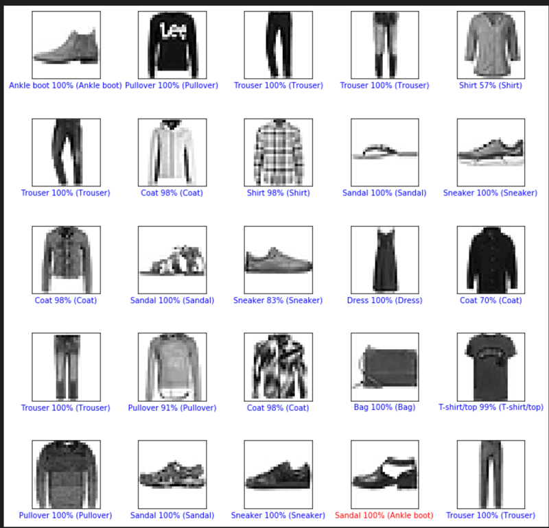
In above output, bottom label of each image has first predicted class and then actual class in parenthesis. You can see second last prediction was wrong and rest predictions are correct.

Conclusion

In this article, we saw the basics of convolutional neural networks, how it works. Also, learned how to build a CNN model, evaluate it, and use it to predict images using tf.Keras API in TensorFlow 2. Also,we checked the impact of CNN in model test accuracy.

Enjoy TensorFlow !!