This article will explain brief summary of linear regression and how to implement it using TensorFlow 2. If you are beginner, I would recommend to read following posts first:
- Setup Deep Learning environment: Tensorflow, Jupyter Notebook and VSCode
- Tensorflow 2: Build Your First Machine Learning Model with tf.keras
Regression
It is a process where a model learns to predict a continuous value output for a given input data. For example, we are given some data points of x and corresponding y and we need to learn the relationship between them that is called a hypothesis.
In case of Linear regression, the hypothesis is a straight line, i.e, the response value(y) as accurately as possible as a function of the feature or independent variable(x).
y = W*x + b
Where W is a vector called Weights and b is a scalar called Bias. The Weights and Bias are called the parameters of the model.
Simple Example
Let us consider a dataset where we have a value of response y for every feature x:
| X | Y |
|---|---|
| 0 | 5 |
| 1 | 8 |
| 2 | 11 |
| 3 | 14 |
| 4 | 17 |
| 5 | 20 |
| 6 | 23 |
| 7 | 26 |
| 8 | 29 |
| 9 | 32 |
We have to predict value for x=10
Let's build Tensorflow 2 model for this:
import tensorflow as tf

x = [0, 1, 2, 3, 4, 5, 6, 7, 8, 9]
y = [5, 8, 11, 14, 17, 20, 23, 26, 29, 32]

# Define layer
layer0 = tf.keras.layers.Dense(units=1, input_shape=[1])

model = tf.keras.Sequential([layer0])

# Compile model
model.compile(loss='mean_squared_error',
              optimizer=tf.keras.optimizers.Adam(1))

# Train the model
history = model.fit(x, y, epochs=100, verbose=False)

# Prediction
print('Prediction: {}'.format(model.predict([10])))

# Get weight and bias
weights = layer0.get_weights()
print('weight: {} bias: {}'.format(weights[0], weights[1]))
In above code, we defined x and y with provided data. then define keras Dense layer with single Neuron and compiled the model with mean squared error and Adam optimizer. After training, we define to get prediction for x=10 and display to check weight and bias.
Here is the output
Prediction: [[35.]]
weight: [[3.]] bias: [5.]
Which is correct. As it is very simple example for understanding purpose.
y = W*x + b
y = 3x + 5
for x= 0, y=5
x=1, y = 8
...
x=10, y= 3*10+5 = 35
Another Example
Let's prepare a linear dataset
import numpy as np
import tensorflow as tf
import matplotlib.pyplot as plt
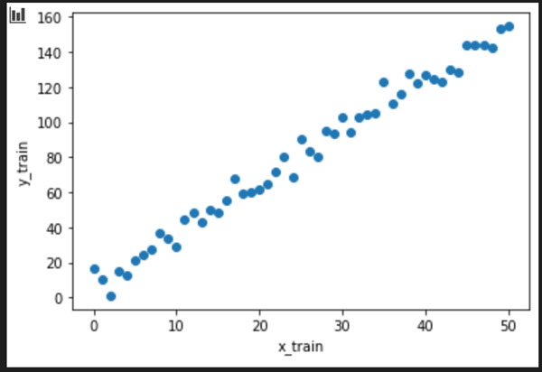
x_train = np.linspace(0, 50, 51)
y_train = np.linspace(5, 155, 51)
It is similar to previous one ((x,y)(0,5)(1,8)(2,11)...) except total number of data points. Let's add some noise:
y_train = y_train + np.random.normal(0,5,51)
Let's visualize the training data
plt.xlabel('x_train')
plt.ylabel('y_train')
plt.scatter(x_train, y_train)
plt.show()
Build the model:
layer0 = tf.keras.layers.Dense(units=1, input_shape=[1])

model = tf.keras.Sequential([layer0])

model.compile(loss='mean_squared_error',
              optimizer=tf.keras.optimizers.Adam(0.1))

history = model.fit(x_train,y_train, epochs=100, verbose=False)
The model is similar to previous except Adam arg value.
Check the training loss:
plt.xlabel('Epoch Number')
plt.ylabel("Loss Magnitude")
plt.plot(history.history['loss'])
plt.show()
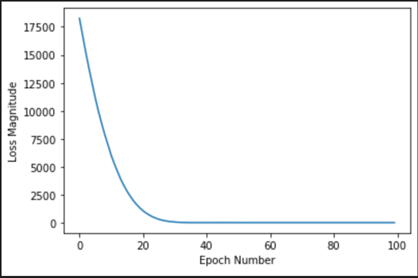
As you can see, our model improves very quickly at first, and then has a steady, slow improvement until it is very near "perfect" towards the end.
Let's get prediction for x=100
print('Prediction: {}'.format(model.predict([100])))
Output:
Prediction: [[304.8801]]
Which is ~305. Let's plot the result
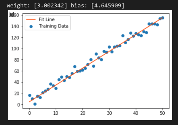
weights = layer0.get_weights()
weight = weights[0][0]
bias = weights[1]
print('weight: {} bias: {}'.format(weight, bias))
y_learned = x_train * weight + bias
plt.scatter(x_train, y_train, label='Training Data')
plt.plot(x_train, y_learned, color='orangered', label='Fit Line')
plt.legend()
plt.show()
Conclusion
In this article, we saw what is linear regression with a very simple example and learned how to build a linear regression model, evaluate it, and use it to predict new data values using TensorFlow 2.0 Keras API.
Enjoy TensorFlow!!